Measures of central tendency

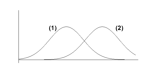
Characteristics of Distributions

Central Tendency (or Location)

Arithmetic Mean
This is the most useful of the three measures of location. If  are  observations on a variable X then the arithmetic mean , is defined as:

 
i.e. 

 
i.e. 

(i) when the classes are individual discrete values as in the radiation data:
 

(i) The thickness of the magnetic coating was measured at 10 randomly chosen points on the surface of a flexible disc produced by a manufacturer. The following results, in microns  were obtained.

Thickness     973     975     976     977     976     980     981     977     979     976

The mean thickness is given by  977 microns

(ii) We have already met the following data on the heights of trees
 

Height (cms)	Frequency (f)	Class midpoint
49.5 - 79.5	7	64.5
79.5 - 109.5	11	94.5
109.5 - 139.5	14	124.5
139.5 - 169.5	21	154.5
169.5 - 199.5	42	184.5
199.5 - 229.5	35	214.5
229.5 - 259.5	10	244.5
	140

The Median

(a) Discrete Distribution
Consider a set of data on a discrete variable. Arrange the data in ascending or descending order of magnitude then the median is: (i) the middle item for an odd number of observations, (ii) the average of the two middle items for an even number of observations.  In general if there are n observations the median is the value of th observation .
For example:

2,     5,     6,     8,     13,     15,     19,     22,     38     have median 13
3,     4,     8,     9,     13,     16,     17,     20,     21,     22     have median  i.e. 14.5

The main difference between the median and the mean is that the median is insensitive to extreme values since, unlike the arithmetic mean, it does not take into account the actual value of each observation, but only considers the rank of each measurement.

The median is useful in such areas as lifetime testing of components.

Quartiles
The upper and lower quartiles (together with the median) divide the observations into quarters.  For n observations on a discrete variable the upper and lower quartiles are the values of the  and the  observations respectively when they are arranged in ascending order of magnitude.

For a distribution on a continuous variable the quartiles are, like the median, easy to estimate from the ogive by drawing lines across at 25% and 75% on the vertival scale and then down to the horizontal scale and reading them off (again see the picture above of the ogive).

The Mode
The MODE of a set of observations is the value that occurs most frequently.  When designating the mode for a grouped frequency distribution, we usually refer to the MODAL CLASS, where the modal class is the class with the highest frequency. If a single value for the mode of grouped data must be specified, it is taken as the midpoint of the modal class.

For example, for the data on the height of nine year old trees, the modal class is 169.5 -199.5(cm) so that 184.5 cm would be taken as the mode.

The disadvantage with the mode as a measure of location is that it is not always unique, ie a distribution can have more than one mode.

For grouped data the mode is not uniquely defined, since changing the class intervals may give different maximum frequencies.

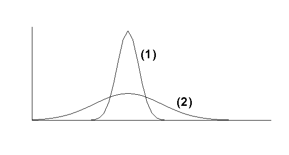
Dispersion (Spread or Scatter)

The Range
The RANGE of a set of observations is the difference between the greatest and least of the observations. It is easy to calculate and is widely used in industrial quality control as one check on manufactured items. However, it ignores the distribution of the observations between the extremes (eg possible concentrations about the centre) and is too easily affected by freak results.

For example:     2.3     4.1     5.2     6.9     8.8     9.4   have range = 9.4 - 2.3 = 7.1.
Also                  2.3     6.1     6.2     6.4     6.6     9.4   still have range 7.1