
Measures of dispersal/spread
Characteristics of Distributions
Dispersion (Spread or Scatter)
The Range
The RANGE of a set of observations is the difference
between the greatest and least of the observations. It is easy to calculate and
is widely used in industrial quality control as one check on manufactured items.
However, it ignores the distribution of the observations between the extremes
(eg possible concentrations about the centre) and is too easily affected by
freak results.
For example: 2.3 4.1 5.2 6.9 8.8 9.4 have range = 9.4 - 2.3 = 7.1.Semi-Interquartile Range
Also 2.3 6.1 6.2 6.4 6.6 9.4 still have range 7.1
This is defined as: siqr = ½ (upper quartile - lower quartile)
Again this is fairly easy to calculate, is not so easily affected by freak results and is useful for comparing the dispersion of similarly shaped distributions.
Variance and Standard Deviation
Ideally, a
measure which uses all the observed data to calculate some average deviation
from the centre of the distribution would be preferred to both of the above
quantities.
Consider the following two simple distributions:
both have the same mean value yet the8 9 9 11 13

2 4 9 11 24
Nothing is gained by considering the mean of these differences as a measure of spread since-2 -1 -1 1 3
-8 -6 -1 1 14
This can be overcome by considering the mean of the numerical deviations of the observations from their mean, ie ignoring whether these deviations are negative or positive, defining

mean deviation = 
for the above distributions
mean deviation for the2 1 1 1 3
8 6 1 1 14
However, this quantity is not suitable for algebraic manipulation and the elimination of the negative signs of the deviations is best achieved by squaring and then finding the mean of these squares, ie defining:
variance 
To obtain a measure of dispersion having the same units as the original variable we define4 1 1 1 9
64 36 1 1 196
variance for thevalues =

variance for thevalues =
standard deviation ![]()
 .
.
Standard deviation for the ![]() values
values ![]() and
and
standard deviation for the ![]() values
values ![]()
Again the statistics facilities of your calculator can be used to find the standard deviation. However, most calculators have two versions for the standard deviation. These are:
(the one we have already seen) and. . . . . . (1)
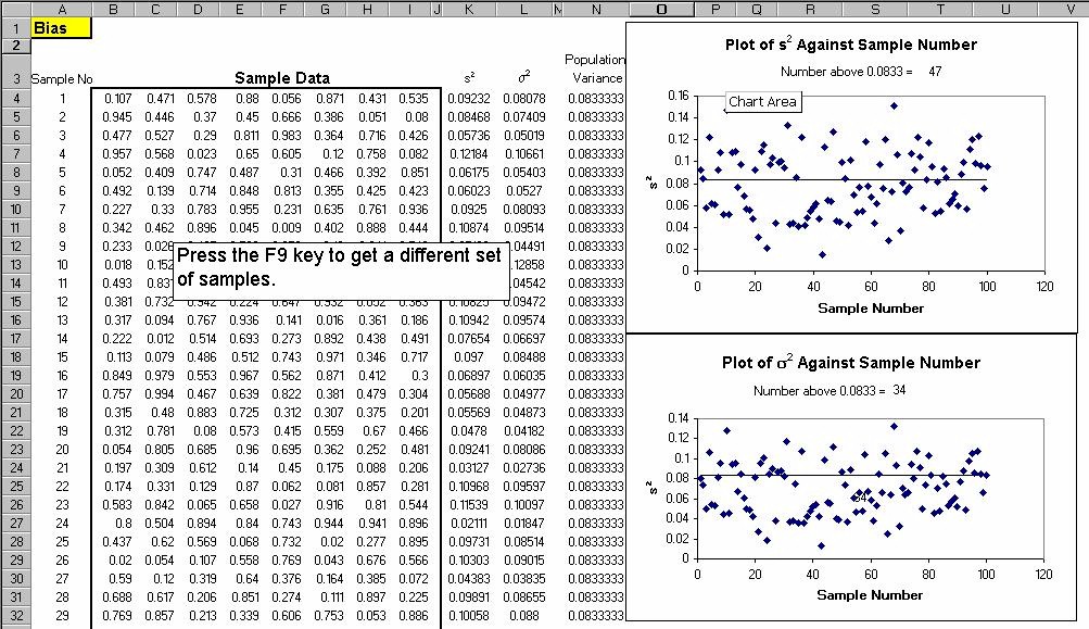
Expression (1) is the standard deviation of a set of data values which constitute the totality of those values in which we are interested, ie the population. As already mentioned we are rarely able to study the population exhaustively so s can not often be calculated. Calculating s from all possible samples from a given population and then finding their average produces a value which is smaller than the population standard deviation. Consequently expression (1) is said to produce a biased estimate of the population standard deviation.. . . . . . (2)
It can be shown that changing the divisor n in expression (1) to n-1 to give expression (2) produces an estimate the standard deviation of a population, of which the n data values are a random sample, which is unbiased. Consequently s is the value usually calculated.
Some texts use ![]() instead of s for expression (2), the symbol
instead of s for expression (2), the symbol ![]() denoting that the quantity is an estimator. Some calculators
represent expression (1) by
denoting that the quantity is an estimator. Some calculators
represent expression (1) by ![]() and expression (2) by
and expression (2) by ![]() whilst others actually use
whilst others actually use ![]() and s.
and s.
Below is a demonstration of bias in which 100 samples are taken from a uniform (0,1) distribution and
Example
Consider again the data on the thickness of the magnetic coating on the flexible disc, ie
973 975 976 977 976 980 981 977 979 976
Use your calculator to confirm that s, the estimated standard deviation of the population from which this sample is taken is = 2.40 microns.
For grouped data the expressions for the standard deviation become
and
Example
Again using the data on the
heights of 140 nine year old trees of a certain species, ie
| Height (cms) |
Class midpoint ( |
Frequency (f) |
| 49.5 - 79.5 | 64.5 |
|
| 79.5 - 109.5 | 94.5 |
|
| 109.5 - 139.5 | 124.5 |
|
| 139.5 - 169.5 | 154.5 |
|
| 169.5 - 199.5 | 184.5 |
|
| 199.5 - 229.5 | 214.5 |
|
| 229.5 - 259.5 | 244.5 |
|
Use your calculator to obtain
The Coefficient of Variation
The
COEFFICIENT OF VARIATION is defined as
As a measure of variability the standard deviation has magnitude which depends on the magnitude of the data.
or(as a percentage)
The COEFFICIENT OF VARIATION expresses sample variability relative to
the mean of the sample. Since s and ![]() have the same units, V has no units at all, a fact which emphasises
that it is a relative measure.
have the same units, V has no units at all, a fact which emphasises
that it is a relative measure.
Example
In order to monitor atmospheric
pollution levels, the amount of SO2 in the atmosphere was
measured in ( gm-3) at eight locations in a certain town.
Measurements were made at the height of summer and the depths of winter giving
the following results:
Summer 25.1 27.2 24.8 29.5 22.7 28.3 23.2 24.6
Winter 43.2 37.5 52.8 61.0 41.7 39.8 65.4 38.1
For summer ![]() 25.7, s = 2.42
25.7, s = 2.42 ![]()
![]() 9.43
9.43
For winter ![]() 47.4, s = 10.89
47.4, s = 10.89 ![]()
![]() 22.96
22.96